G(V,X) with loops but no multiple arcs defines a binary relation X on the set V. The complete graph corresponds to the universal relation. An undirected graph corresponds to a symmetric relation. The complement of the graph corresponds to the complement of the relation. Changing the direction of the arcs corresponds to the reverse relationship.
Digraphs and binary relations are the same class of objects described by different means. Binary relations, functions are the basic tools for building the vast majority of mathematical models that are used to solve practical problems, and graphs can be visualized in the form of a diagram. This explains the widespread use of diagrams of various types in coding and design.
The vertex b of the digraph (graph) G is called achievable from U if and only if U=V or there is a path (route) connecting U with V (U is the initial vertex, V is the final vertex). Thus, on the set of vertices of a digraph (graph), not only the adjacency relation A is defined, but also the reachability relation T.
Reachability matrix T digraph (graph) G is called T 2 n×n, whose elements are found from the condition: 1, if it is reachable from ; 0 if not reachable from .
Definition of the reachability matrix of a digraph as a matrix of reflexive and transitive closure of the adjacency relation.
The introduced relation of reachability at the vertices of the graph G(V,X): the vertex w is reachable from the vertex v if v = w or there is a path from v to w in G. In other words, reachability is the reflexive and transitive closure of the adjacency relation.
Find adjacency matrix, transitive and reflexive closure.
Connectivity in graphs. Weak, one-way and strong connectivity in digraphs. Matrix of connectivity and strong connectivity. Connectivity components. Definition of a matrix of strong connectivity based on the reachability matrix.
G(V,X) is called connected if any of its vertices is reachable from any other vertex.
The digraph G(V,X) is called one way connected, if for any two of its vertices, at least one is reachable from the other.
The digraph G(V,X) is called strongly connected if any of its vertices is reachable from any other.
The digraph G(V,X) is called loosely connected, if the non-digraph corresponding to it, obtained as a result of deleting the orientation of the arcs, is connected.
A digraph that is not weakly connected is called incoherent.
Strong bond component of the digraph G(V,X) is called the maximal, according to the number of occurrences of vertices, strongly connected subgraph of this digraph. The connected component of a non-digraph is defined similarly.
The matrix of strong connectivity (connectivity) of the digraph (graph) G(V,Х) is called S n×n, the elements of which are found from the condition: 1, if it is reachable from and reachable from ; 0 if not reachable from and not reachable from .
(digraph) strongly connected or connected, it suffices to determine the presence of 0 in the matrix if
0 is not present, then the graph (digraph) is connected (strongly connected), otherwise not.
The strongly connected matrix can be constructed from the reachability matrix by the formula
The questions of reachability for digraphs and methods for finding the reachability and counterreachability matrices are considered. A matrix method is considered for finding the number of paths between any vertices of a graph, as well as finding the set of vertices included in the path between a pair of vertices. The purpose of the lecture: To give an idea of reachability and counterreachability and how to find them
Reachability and Counterreachability
Tasks in which the concept is used reachability, quite a bit of.
Here is one of them. Graph may be a model of some organization in which people are represented by vertices, and arcs interpret communication channels. When considering such a model, one can ask whether information from one person i can be transferred to another person j , i.e., is there a path going from vertices i to vertices j . If such a path exists, then we say that the vertices j achievable from vertices i . One can be interested in the reachability of vertices j from vertices i only on paths whose lengths do not exceed a given value or whose length is less than the largest number of vertices in the graph, etc. of the problem.
The reachability in the graph is described by the reachability matrix R=, i, j=1, 2, ... n, where n is the number of graph vertices, and each element is defined as follows:
r ij =1, if vertices j are reachable from x i ,
r ij =0, otherwise.
The set of vertices R(x i) of the graph G, reachable from a given vertex x i , consists of elements x i for which the (i, j)-th element in the reachability matrix is equal to 1. Obviously, all diagonal elements in the matrix R are equal to 1, since each vertex is reachable from itself by a path of length 0. Since the first-order direct mapping Г +1 (x i) is the set of such vertices x j that are reachable from x i using paths of length 1, then the set Г + (Г +1 (x i)) = Г +2 (x i) consists of vertices reachable from x i using paths of length 2. Similarly, r + p (x i) is the set of vertices that are reachable from x i using paths of length p.
Since any graph vertex that is reachable from x i must be reachable using a path (or paths) of length 0 or 1, or 2, ..., or p, then the set of vertices reachable for vertex x i can be represented as
R (x i) = ( x i ) G +1 (x i) G +2 (x i) ... G + p (x i).
As you can see, the set of reachable vertices R(x i) is a direct transitive closure of the vertex x i , i.e. R(x i) = T + (x i). Therefore, to construct the reachability matrix, we find reachable sets R(x i) for all vertices x i X. Setting r ij =1 if x j R(x i) and r ij =0 otherwise.
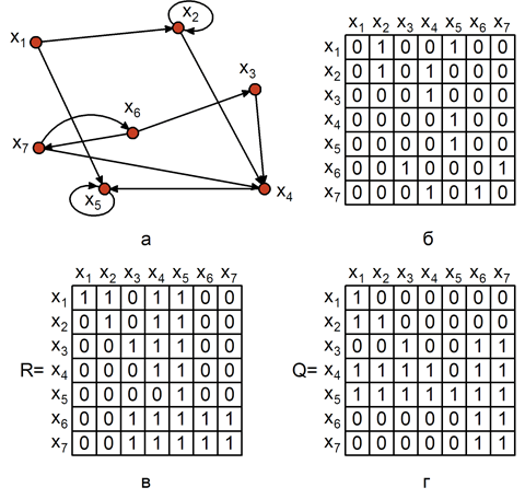
Rice. 4.1. Reachability in the graph: a - graph; b – adjacency matrix; c – reachability matrix; r is the counterreachability matrix.
For the graph shown in fig. 4.1, a, reachable sets are located as follows:
R (x 1) = ( x 1 ) ( x 2 , x 5 ) ( x 2 , x 4 , x 5 ) ( x 2 , x 4 , x 5 ) = ( x 1 , x 2 , x 4 , x 5 ),
R (x 2) = ( x 2 ) ( x 2 , x 4 ) ( x 2 , x 4 , x 5 ) ( x 2 , x 4 , x 5 ) = ( x 2 , x 4 , x 5 ),
R (x 3) = ( x 3 )( x 4 )( x 5 )( x 5 ) = ( x 3 , x 4 , x 5 ),
R (x 4) = ( x 4 )( x 5 )( x 5 ) = ( x 4 , x 5 ),
R (x 5) = ( x 5 )( x 5 ) = ( x 5 ),
R (x 6) = ( x 6 )( x 3 , x 7 )( x 4 , x 6 )( x 3 , x 5 , x 7 )( x 4 , x 5 , x 6 ) = ( x 3 , x 4, x 5, x 6, x 7),
R (x 7) = ( x 7 )( x 4 , x 6 )( x 3 , x 5 , x 7 )( x 4 , x 5 , x 6 ) = ( x 3 , x 4 , x 5 , x 6 , x 7 ).
Reachability matrix has the form as shown in Fig. 4.1, c. Reachability matrix can be built according adjacency matrix(Fig. 4.1b), forming setsT + (x i) for each vertex x i .
Counterreachability matrix Q = [ q ij ],i, j =1, 2, ... n, where n is the number of graph vertices, is defined as follows:
q ij =1, if from vertex x j it is possible to reach vertex x i ,
q ij =0, otherwise.
counterachievable the set Q (x i) is the set of vertices such that from any vertex of this set it is possible to reach the vertex x i . Similarly to the construction of the reachable set R (x i), we can write an expression for Q (x i):
Q (x i) = ( x i ) Г -1 (x i) Г - 2(x i) ... Г -p (x i).
Thus, it is clear that Q (x i) is nothing more than the reverse transitive closure of the vertex x i, i.e. Q (x i) = T - (x i). It is obvious from the definitions that the column x i of the matrix Q (in which q ij =1 if x j Q (x i), and q ij =0 otherwise) coincides with the row x i of the matrix R, i.e., Q = R T , where R T is the matrix transposed to reachability matrix R.
Counterreachability matrix shown in fig. 4.1, g.
It should be noted that since all elements of the matrices R and Q are equal to 1 or 0, each row can be stored in binary form, saving computer memory costs. Matrices R and Q are convenient for processing on a computer, since from a computational point of view, the main operations are high-speed logical operations.
Finding the set of vertices included in the path
If you need to know about the vertices of the graph included in these paths, then you should remember the definitions of direct and inverse transitive closures. Since T + (x i) is the set of vertices to which there are paths from the vertex x i , and T - (x j) is the set of vertices from which there are paths to x j , then T + (x i) T - (x j) is the set of vertices , each of which belongs to at least one path going from x i to x j . These vertices are called essential or integral with respect to the two end vertices x i and x j . All other vertices of the graph are called insignificant or redundant, since their removal does not affect the paths from x i to x j .

Rice. 4.2. digraph
So for the graph in Fig. 4.2 finding the vertices included in the path, for example, from vertex x 2 to vertices 4, is reduced to finding T + (x 2) \u003d ( x 2, x 3, x 4, x 5, x 6 ),
T - (x 4) \u003d ( x 1, x 2, x 3, x 4, x 5), and their intersections T + (x 2) T - (x 4) \u003d ( x 2, x 3, x 4, x 5 ).
Matrix method for finding paths in graphs
The adjacency matrix completely defines the structure of the graph. Let's square the adjacency matrix according to the rules of mathematics. Each element of the matrix A 2 is determined by the formula
a (2) ik = n j=1 a ij a jk
The term in the formula is equal to 1 if and only if both numbers a ij and a jk are equal to 1, otherwise it is equal to 0. Since the equality a ij = a jk = 1 implies the existence of a path of length 2 from vertex x i to vertices k passing through vertex x j , then the (i -th,k-th) element of the matrix A 2 is equal to the number of paths of length 2 going from x i to k .
Table 4.1a shows the adjacency matrix of the graph shown in fig. 4.2. The result of squaring the adjacency matrix A 2 is shown in Table 4.1b.

So "1", standing at the intersection of the second row and the fourth column, indicates the existence of one path of length 2 from vertex x 2 to vertices 4 . Indeed, as we see in column in fig. 4.2, there is such a path: a 6 , a 5 . The "2" in matrix A 2 indicates the existence of two paths of length 2 from vertices 3 to vertices 6: a 8 , a 4 and a 10 , a 3 .
Similarly, for the adjacency matrix raised to the third power A 3 (Table 4.1c), a (3) ik is equal to the number of paths of length 3 going from x i to x k . It can be seen from the fourth row of matrix A 3 that there are paths of length 3: one of x 4 in 4 (a 9 , a 8 , a 5), one of x 4 in
x 5 (a 9, a 10, a 6) and two paths from x 4 in 6 (a 9, a 10, a 3 and a 9, a 8, a 4). Matrix A 4 shows the existence of paths of length 4 (Table 4.1d).
Thus, if a p ik is an element of the matrix A p, then a p ik is equal to the number of paths (not necessarily or chains or simple or chains) of length p going from x i to x k .
REACHABILITY AND CONNECTIVITY IN GRAPHS Lecture outline: Paths of a chain and cycles. Graph connectivity and connectivity components. Diameter, radius and center of the graph.
Share work on social networks
If this work does not suit you, there is a list of similar works at the bottom of the page. You can also use the search button
Baranov Viktor Pavlovich Discrete Math. Section 3Graphs, networks, codes.
Lecture 8
Lecture 8 REACHABILITY AND CONNECTIVITY IN GRAPHS
Lecture plan:
- Routes, chains and cycles.
- Graph connectivity and connectivity components.
- Diameter, radius and center of the graph.
- Reachability and counterreachability matrices.
- Routes, circuits and loops
Oriented route(or by ) of a digraph is a sequence of arcs in which the end vertex of any arc other than the last one is the starting vertex of the next one. On fig. 1 arc sequence
, (1)
, (2)
(3)
are paths.
Rice. one.
oriented chain(or orepio ) is called the path in which each arc and with used no more than once. So, for example, paths (2) and (3) are orchains, but path (1) is not, since the arc is used twice in it.
Simple is called a chain in which each vertex is used by at most one about times. For example, orchain (3) is simple, but orchain (2) is not.
Route is an undirected twin of the path, i.e., a sequence of edges in which each edge, except for the first and last, is connected by end vertices with the edges and. A bar over an arc symbol means that it is treated as an edge.
Just as we have defined orchains and simple chains, we can define chains and simple chains.
A path or route can also be represented by a sequence of vertices. For example and measures, path (1) can be written as: .
The path is called closed , if the initial vertex of the arc in it coincides with the horse h noah apex of the arc. Closed orchains (chains) are called orcycles (cycles ). Orcycles are also called contours . Closed simple orchains (chains) called s simple orcycles(cycles). closed routeis unoriented n closed double at you.
- Graph Connectivity and Connectivity Components
A vertex in a digraph is said to be reachable from the vertex if there is a path. If, moreover, is reachable from, then these vertices are said to be mutually reachable.
A digraph is called strongly connected or strong , if any two vertices in it are a imo achievable. An example of a strong digraph is shown in fig. 2 a. Since in the column e given an orcycle that includes all vertices, then any two of them are taken but achievable.
° ° °
° ° ° ° ° °
° ° ° ° ° °
a B C
Rice. 2.
The digraph is calledone way connected or unilateral if in any pair of its vertices at least one is reachable from the other. An example of a one-way graph is shown in fig. 2 b. This graph has an orcycle that includes four mutually reachable vertices. The vertex has a degree of entry of zero, which means that there are no paths leading to this vertex. Moreover, any of the other four vertices is reachable from it.
The digraph is called loosely connected or weak , if it contains any two vertices with about united halfway . A half path, unlike a path, can have the opposite direction. in lazy arcs. An example of a weak digraph is shown in fig. 2 in. It is obvious that the graph does not contain at ty between the vertices and, but there is a half-path consisting of opposite n a ruled arcs and.
If for some pair of vertices there is no route connecting them, then t a which digraph is called incoherent.
Three types of connected components are defined for a digraph:strong component– ma k the strongest subgraph,one-sided component- maximum single about ronny subgraph andweak componentis the weakest subgraph.
The concept of a strong component is illustrated in Fig. 3.
° ° ° ° ° °
° ° ° °
° ° ° ° ° °
° ° ° ° ° °
° ° °
° ° ° ° °
Rice. 3
A graph that is unidirectionally connected contains six strong d graphs, of which only and are strong components n tami. The concept of a one-way component is illustrated similarly. In this note e The re one-way component is the same as the graph itself. If we change the orientation a arc, for example, to the opposite one, then we get a weak graph with two one-sided about frontal components, one of which is formed by vertices, and the other by ve r tires.
For an undirected graph, we define on the set of its vertices the bin R relation, assuming if there is a chain linking to. This relation is a gives the properties of reflexivity, symmetry and transitivity, that is, it is about t wearing equivalence. It splits the set of vertices into non-intersecting classes: . Two vertices from the same class are equivalent, that is, there is a chain in the graph that connects them; there is no such chain for vertices from different classes. Since the ends of Yu If the edges are in relation, then the set of edges of the graph will also be divided into non-intersecting classes: , where the set of all edges whose ends belong to is denoted by .
The graphs are connected and add up to a graph. These graphs are calledconnectivity componentsgraph. A number is another numerical characteristic of a graph. For a connected graph, if the graph is disconnected, then.
If the given graph is not connected and splits into several components, then the solution of any question regarding this graph, as a rule, can be reduced to the study of individual components that are connected. Therefore, in most cases it makes sense to assume that the given graph is connected.
- Diameter, radius and graph center
For a connected graph, we define distance between its two vertices and as the length of the shortest chain connecting these vertices, and denoted by. The length of a chain is the number of edges that make up the chain. It is easy to check that you enter n This distance satisfies the axioms of the metric:
2) ;
3) .
Determine the distance from each vertex of the graph to the vertex farthest from it
which is calledeccentricity. Obviously, the eccentricity for all vertices in the complete graph is equal to one, and for the vertices of a simple cycle - .
The maximum eccentricity is called diameter graph, and the minimum - radius graph. In the full graph we have, and in a simple cycle - .
A vertex is called central if. The graph may have several b such vertices, and in some graphs all vertices are central. In a simple chain, with an odd number of vertices, only one is central, and with an even number of them with there are two such vertices. In a complete graph and for a simple cycle, all vertices are central. The set of central vertices is called the center of the graph.
Example 1 Find the diameter, radius and center of the graph shown in fig. 4.
° °
° ° °
° °
° °
Rice. 4.
To solve this problem, it is convenient to precomputedistance matrix between the tops mi count. In this case, it will be a matrix of size, in which the distance from vertex to vertex is in place:
For each row of the matrix, we find the largest element and write it down with a wa from the dash. The largest of these numbers is equal to the diameter of the graph, the smallest is p a the graph's dius. The center of the graph is formed by the central vertices and.
The concepts of the central vertex and the center of the graph appeared in connection with the problems of optimism. and small location of public service points, such as hospitals, fire departments, public order stations, etc., when it is important to minimize the and greater distance from any point of some network to the nearest service point a niya.
- Reachability and counterreachability matrices
Reachability matrixis defined as follows:
The set of graph vertices reachable from a given vertex consists of those elements for which the th element in the matrix is equal to 1. This set can be represented as
Counterreachability matrix (inverse reachability) define is as follows:
Similarly to the construction of an accessible set, one can form a set about gesture using the following expression:
It follows from the definitions that the -th column of the matrix coincides with the -th row of the ma t , i.e. , where is the matrix transposed to the matrix.
Example 2 Find matrices of reachability and counterreachability for a graph, etc. and shown in Fig. 5.
Rice. 5.
Let us define the reachability sets for graph vertices:
Therefore, the reachability and counterreachability matrices have the form:
Since is the set of such vertices, each of which belongs to at least one path going from to, then the vertices of this set are called are essential or inalienable with respect to the end vertices and. All other vertices are calledinsignificant or redundant , since their removal does not affect the paths from to.
You can also define matrices limited reachability and counterreachability and bridges, if we require that the lengths of the paths do not exceed some given number. Then will be the upper bound on the length of admissible paths.
The graph is said to be transitive if from the existence of arcs and the trace at there is the existence of an arc.transitive closuregraph is a graph, where is the minimum possible set of arcs necessary for the graph to be transitive. It is obvious that the reachability matrix of the graph coincides with the adjacency matrix of the graph, if we put units on the main diagonal in the matrix.
Reachability Graph
One of the first questions that arise in the study of graphs is the question of the existence of paths between given or all pairs of vertices. The answer to this question is the above relation of reachability at the vertices of the graph G=(V,E): the vertex w is reachable from the vertex v if v = w or there is a path from v to w in G. In other words, the reachability relation is the reflexive and transitive closure of the relation E. For undirected graphs, this relation is also symmetric and, therefore, is an equivalence relation on the vertex set V. In an undirected graph, reachability equivalence classes are called connected components. For directed graphs, reachability does not, in general, have to be a symmetric relation. Mutual reachability is symmetric.
Definition 9.8. Vertices v and w of a directed graph G=(V,E) are said to be mutually reachable if G has a path from v to w and a path from w to v.
It is clear that the mutual reachability relation is reflexive, symmetric, and transitive, and hence an equivalence on the vertex set of the graph. Equivalence classes with respect to mutual reachability are called strongly connected components or doubly connected components graph.
Let us first consider the question of constructing the reachability relation. Let us define for each graph its reachability graph (sometimes also called the transitive closure graph), whose edges correspond to the paths of the original graph.
Definition 9.9. Let G=(V,E) be a directed graph. The reachability graph G * =(V,E *) for G has the same set of vertices V and the following set of edges E * =( (u, v) | in the graph G, the vertex v is reachable from the vertex u).
Example 9.3. Consider the graph G from Example 9.2.
Rice. 9.2. Count G
Then we can check that the reachability graph G* for G looks like this (new loop edges at each of the vertices 1-5 are not shown):

Rice. 9.3. Count G*
How can a graph G * be constructed from a graph G? One way is to determine for each vertex of the graph G the set of vertices reachable from it by sequentially adding to it the vertices reachable from it by paths of length 0, 1, 2, and so on.
We will consider another method based on the use of the adjacency matrix A G of the graph G and Boolean operations. Let the set of vertices V=(v 1 , … , v n ). Then the matrix A G is an n × n Boolean matrix.
Below, in order to preserve the similarity with the usual operations on matrices, we will use "arithmetic" notation for Boolean operations: by + we will denote disjunction , and by · - conjunction .
Denote by E n the identity matrix of size n × n. Let's put ![]() . Let Our procedure for constructing G * be based on the following statement.
. Let Our procedure for constructing G * be based on the following statement.
Lemma 9.2. Let be . Then
Proof let us carry out by induction on k.
Basis. For k=0 and k=1, the statement is true by definition and .
induction step. Let the lemma be valid for k. Let us show that it remains valid for k + 1 as well. By definition we have:
Assume that in the graph G from v i to v j there is a path of length k+1. Consider the shortest of these paths. If its length is k, then by the induction hypothesis a_(ij)^((k))=1. In addition, a jj (1) =1. Therefore a ij (k) a jj (1) =1 and a ij (k+1) =1. If the length of the shortest path from v i to v j is equal to k+1, then let v r be its penultimate vertex. Then from v i to v r there is a path of length k and, by the induction hypothesis, a ir (k) =1. Since (v r ,v j) E, then a_(rj)^((1))=1. Therefore a ir (k) a rj (1) =1 and a ij (k+1) =1.
Conversely, if a ij (k+1) =1, then for at least one r the summand a ir (k) a rj (1) is equal to 1. If this is r=j, then a ij (k) =1 and by the inductive hypothesis, G has a path from v i to v j of length k. If r j, then a ir (k) =1 and a rj (1) =1. This means that G has a path from v i to v r of length k and an edge (v r ,v j) E. Combining them, we get a path from v i to v j of length k+1.
From Lemmas 9.1 and 9.2 we directly obtain
Consequence 1. Let G=(V,E) be a directed graph with n vertices and G * its reachability graph. Then A_(G*) = . Proof. Lemma 5.1 implies that if G has a path from u to v u, then it also has a simple path from u to v of length n-1. And by Lemma 5.2, all such paths are represented in the matrix .
Thus, the procedure for constructing the adjacency matrix A G* of the reachability graph for G is reduced to raising the matrix to the power of n-1. Let us make some remarks to simplify this procedure.
where k is the smallest number such that 2 k n.
such r is found that a ir = 1 and a rj =1, then the whole sum a ij (2) =1. Therefore, the rest of the terms can be ignored.
Example 9.3. Let us consider as an example the calculation of the matrix of the reachability graph A G* for the graph G presented in fig.9.2. In this case

Since G has 6 vertices, then . Let's calculate this matrix:

and (the last equality is easy to check). Thus,

As you can see, this matrix really defines the graph shown in fig.9.3.
Mutual Reachability, Strongly Connected Components, and Graph Bases
By analogy with the reachability graph, we define a graph of strong reachability.
Definition 9.10. Let G=(V,E) be a directed graph. The strongly reachable graph G * * =(V,E * *) for G has the same set of vertices V and the following set of edges E * * =( (u, v) | in G, vertices v and u are mutually reachable).
From the matrix of the reachability graph, it is easy to construct the matrix of the strong reachability graph. Indeed, it follows directly from the definitions of reachability and strong reachability that for all pairs (i,j), 1 i,j n, the value of an element is equal to 1 if and only if both elements A G* (i, j) and A G* (j, i) are equal to 1, i.e.
Based on the matrix, one can single out the strongly connected components of the graph G as follows.
Let us place in the component K 1 the vertex v 1 and all vertices v j such that A_(G_*^*)(1,j) = 1.
Let the components K 1 , …, K i and v k have already been built - this is the vertex with the minimum number that has not yet been included in the components. Then we place in the component K_(i+1) the vertex v k and all such vertices v j ,
that A_(G_*^*)(k,j) = 1.
Repeat step (2) until all vertices are distributed among the components.
In our example, for graph G on fig.2 by the matrix, we obtain the following matrix of the graph of strong reachability

Using the procedure described above, we find that the vertices of the graph G are divided into 4 strongly connected components: K 1 = (v 1 , v 2 , v 3 ), \ K 2 =( v 4 ), \ K 3 =( v 5 ), \ K 4 =( v 6 ). On the set of strongly connected components, we also define the reachability relation.
Definition 9.11. Let K and K" be strongly connected components of a graph G. The component K reachable from components K^\prime if K= K" or there are two vertices u K and v K" such that u is reachable from v. K strictly achievable from K^\prime if K K" and K is reachable from K". The K component is called minimum if it is not strictly reachable from any component.
Since all vertices in one component are mutually reachable, it is easy to see that the relations of reachability and strict reachability on the components do not depend on the choice of vertices u K and v K".
The following characteristic of strict reachability is easily deduced from the definition.
Lemma 9.3. The strict reachability relation is a partial order relation, i.e. it is antireflexive, antisymmetric, and transitive.
This relation can be represented as a directed graph whose vertices are the components, and the edge (K", K) means that K is strictly reachable from K". On the rice. 9.4 this graph of components is shown for the graph G considered above.

Rice. 9.4.
In this case, there is one minimal component K 2 .
In many applications, a directed graph is a distribution network of some resource: product, product, information, etc. In such cases, the problem naturally arises of finding the minimum number of such points (vertices) from which this resource can be delivered to any point in the network.
Definition 9.12. Let G=(V,E) be a directed graph. The subset of vertices W V is called generative, if from the vertices of W it is possible to reach any vertex of the graph. A subset of vertices W V is called a graph base if it is generating, but none of its own subsets is generating.
The following theorem allows one to efficiently find all bases of a graph.
Theorem 9.1. Let G=(V,E) be a directed graph. A subset of vertices W V is a base of G if and only if it contains one vertex from each minimal strongly connected component of G and does not contain any other vertices.
Proof Note first that each vertex of the graph is reachable from a vertex that belongs to some minimal component. Therefore, the set of vertices W containing one vertex from each minimal component is generating, and when any vertex is removed from it, it ceases to be such, since the vertices from the corresponding minimal component become unreachable. Therefore W is a base.
Conversely, if W is a base, then it must include at least one vertex from each minimal component, otherwise the vertices of such a minimal component will be inaccessible. W cannot contain any other vertices, since each of them is reachable from the already included vertices.
This theorem implies the following procedure for constructing one or listing all the bases of the graph G.
Find all strongly connected components of G.
Determine the order on them and select the components that are minimal with respect to this order.
Generate one or all bases of the graph by choosing one vertex from each minimum component.
Example 9.5. We define all bases of the directed graph G shown in fig.9.5.

Rice. 9.5. Count G
At the first stage, we find the strongly connected components of G:
At the second stage, we construct a strict reachability graph on these components.

Rice. 9.6. Reachability relation graph on G components
We determine the minimum components: K 2 = ( b ), K 4 =( d, e, f, g) and K 7 = ( r).
Finally, we list all four bases of G: B 1 = ( b, d, r), B 2 = ( b, e, r), B 3 = ( b, f, r) and B 1 = ( b, g, r) .
Tasks
Problem 9.1. Prove that the sum of the degrees of all vertices of an arbitrary directed graph is even.
This problem has a popular interpretation: to prove that the total number of handshakes exchanged by people who came to the party is always even.
Problem 9.2. List all non-isomorphic undirected graphs that have at most four vertices.
Problem 9.3. Prove that an undirected connected graph remains connected after removing some edge ↔ this edge belongs to some cycle.
Problem 9.4. Prove that an undirected connected graph with n vertices
contains at least n-1 edges,
if it contains more than n-1 edges, then it has at least one cycle.
Problem 9.5. Prove that in any group of 6 people there are three pairwise acquaintances or three pairwise strangers.
Problem 9.6. Prove that the undirected graph G=(V,E) is connected ↔ for each partition V= V 1 V 2 with non-empty V 1 and V 2 there is an edge connecting V 1 with V 2 .
Problem 9.7. Prove that if there are exactly two vertices of odd degree in an undirected graph, then they are connected by a path.
Problem 9.8. Let G=(V,E) be an undirected graph with |E|< |V|-1. Докажите, что тогда G несвязный граф.
Problem 9.9. Prove that any two simple paths of maximum length in a connected undirected graph have a common vertex.
Problem 9.10. Let an undirected graph without loops G=(V,E) have k connected components. Prove that then
Problem 9.11. Define what is a reachability graph for
a graph with n vertices and an empty set of edges;
graph with n vertices: V= (v 1 ,… , v n ), whose edges form a cycle:
Problem 9.12. Compute Reachability Graph Matrix for Graph
and construct the corresponding reachability graph. Find all bases of graph G.
Problem 9.13. Build for given on rice. 9.7 directed graph G 1 =(V,E) its adjacency matrix A G1 , incidence matrix B G1 and adjacency lists. Calculate the reachability matrix A G1* and construct the corresponding reachability graph G 1 * .

Rice. 9.7.
Undirected and oriented trees
Trees are one of the most interesting classes of graphs used to represent various kinds of hierarchical structures.
Definition 10.1. An undirected graph is called a tree if it is connected and has no cycles.
Definition 10.2. A directed graph G=(V,E) is called a (directed) tree if
On the rice. 10.1 examples of an undirected tree G 1 and a directed tree G 2 are shown. Note that the tree G 2 is obtained from G 1 by choosing the vertex c as the root and orienting all edges in the "away from the root" direction.

Rice. 10.1. Undirected and directed trees
This is no coincidence. Prove yourself the following assertion about the connection between undirected and directed trees.
Lemma 10.1. If in any undirected tree G=(V,E) we choose an arbitrary vertex v V as a root and orient all edges in the direction "from the root", i.e. make v the beginning of all edges incident to it, the vertices adjacent to v - beginnings of all not yet directed edges incident to v, etc., then the resulting directed graph G" will be a directed tree.
Undirected and directed trees have many equivalent characteristics.
Theorem 10.1. Let G=(V,E) be an undirected graph. Then the following conditions are equivalent.
G is a tree.
For any two vertices in G, there is a unique path connecting them.
G is connected, but when any edge is removed from E, it ceases to be connected.
G is connected and |E| = |V| -one.
G is acyclic and |E| = |V| -one.
G is acyclic, but adding any edge to E generates a cycle.
Proof(1) (2): If some two vertices in G were connected by two paths, then, obviously, there would be a cycle in G. But this contradicts the definition of a tree in (1).
(2) (3): If G is connected, but E remains connected when some edge (u,v) is removed, then there is a path between u and v that does not contain this edge. But then G has at least two paths connecting u and v, which contradicts condition (2).
(3) (4): Provided to the reader (see problem 9.4).
(4) (5): If G contains a cycle and is connected, then when removing any edge from the cycle, the connectivity should not be broken, but the edges remain |E|= V -2, and by Problem 9.4(a), the connected graph must have at least V -1 ribs. The resulting contradiction shows that there are no cycles in G and condition (5) is satisfied.
(5) (6): Suppose that adding an edge (u,v) to E did not result in a cycle. Then the vertices u and v in G are in different connected components. Since |E|= V -1, then in one of these components, let it be (V 1 ,E 1), the number of edges and the number of vertices are the same: |E 1 |=|V 1 |. But then it contains a cycle (see Problem 9.4(b)), which contradicts the fact that G is acyclic.
(6) (1): If G were not connected, then there would be two vertices u and v from different connected components. Then adding the edge (u,v) to E would not lead to the appearance of a cycle, which contradicts (6). Hence G is connected and is a tree.
For directed trees, it is often convenient to use the following inductive definition.
Definition 10.3. We define by induction a class of directed graphs called trees. At the same time, for each of them, we define a selected vertex - the root.
Rice. 10.2 illustrates this definition.

Rice. 10.2. Inductive definition of directed trees
Theorem 10.2. The definitions of directed trees 10.2 and 10.3 are equivalent.
Proof Let the graph G=(V,E) satisfy the conditions of Definition 10.2. Let us show by induction on the number of vertices |V| that .
If |V|=1, then the only vertex v V is the root of the tree by property (1), i.e. there are no edges in this graph: E = . Then .
Suppose that any graph with n vertices that satisfies Definition 10.2 is included in . Let the graph G=(V,E) with (n+1)-th vertex satisfy the conditions of Definition 10.2. By condition (1), it has a root vertex r 0 . Let k edges emerge from r 0 and they lead to vertices r 1 , … , r k (k 1). Denote by G i ,(i=1, …, k) the graph that includes the vertices V i =( v V|v \textit( reachable from )r i ) and the edges E i E connecting them. It is easy to see that G i satisfies the conditions the conditions of definition 10.2. Indeed, r i does not contain edges, i.e., this vertex is the root of G i . Each of the other vertices from V i has one edge, just like G . If v V i , then it is reachable from the root r i by the definition of the graph G i . Since |V i | n, then by the inductive hypothesis . Then the graph G is obtained by the inductive rule (2) of Definition 10.3 from the trees G 1 , …, G k and therefore belongs to the class .
⇐ If some graph G=(V,E) belongs to the class , then the fulfillment of conditions (1)-(3) of Definition 10.2 for it can be easily established by induction on Definition 10.2. We leave this to the reader as an exercise.
There is a rich terminology associated with oriented trees that comes from two sources: botany and the field of family relations.
A root is the only vertex that does not have edges, leaves are vertices that do not have edges. The path from the root to the leaf is called the branch of the tree. The height of a tree is the maximum length of its branches. The depth of a vertex is the length of the path from the root to that vertex. For a vertex v V, the subgraph of the tree T=(V,E), which includes all vertices reachable from v and the edges from E connecting them, forms a subtree T v of the tree T with root v (see Problem 10.3). The height of v is the height of the tree T v . A graph that is a union of several non-intersecting trees is called a forest.
If an edge leads from vertex v to vertex w, then v is called father w, and w - son v (recently, an asexual pair of terms has been used in English-language literature: parent - child). It follows directly from the definition of a tree that every vertex has a unique father besides the root. If a path leads from vertex v to vertex w, then v is called an ancestor of w, and w is called a descendant of v. Vertices that have a common father are called brothers or sisters.
We single out one more class of graphs that generalizes directed trees - directed acyclic ones. Two types of such labeled graphs will be used below to represent Boolean functions. These graphs can have several roots - vertices that do not include edges, and each vertex can have several edges, and not one, as in trees.
computer technology, in particular program ... 2009 of the year Primary school is an experimental site on introduction of the Federal state ...
M ONITORING MEDIA Modernization of vocational education March - August 2011
SummaryUnited state exams" on choice": informational computertechnology, biology and literature. By the way, in this year USE... question"On the results of the implementation programs development of national research universities in 2009 -2010 years". ...
STRATEGIC DEVELOPMENT PROGRAM Tver 2011
ProgramAT 2009 year. Structural shifts observed in 2010 yearon towards 2009 , ... Professionally – oriented foreign language”, “Modern educational technology". In each program advanced training module " State ...
By analogy with the reachability graph, we define a graph of strong reachability.
Definition:
Let be a directed graph. Strong Reachability Graph for
for  also has many vertices
  and the next set of edges
  in the column
  peaks
peaks  and
and  mutually accessible.
By Reachability Graph Matrix  easy to build a matrix
  graph of strong reachability. Indeed, it follows directly from the definitions of reachability and strong reachability that for all pairs
  ,
, , element value
  equals 1 if and only if both elements
  and
and  are equal to 1, i.e.
By matrix  one can single out the strongly connected components of the graph
  in the following way:

Repeat the second step until all the vertices are distributed among the components.
In our example for the graph  example 14.1. by matrix
  we obtain the following matrix of the graph of strong reachability

Using the procedure described above, we find that the vertices of the graph  are divided into 4 strongly connected components:
  ,
, ,
, ,
, . On the set of strongly connected components, we also define the reachability relation.
Definition:
Let be  and
and  are strongly connected components of the graph
  . Component
  achievable from a component
  , if
, if  or there are two such vertices
  and
and  , what
  reachable from
  .
. strictly achievable from
  , if
, if  and
and  reachable from
  . Component
  is called minimal if it is not strictly reachable from any component.
Since all vertices in one component are mutually reachable, it is easy to understand that the relations of reachability and strict reachability on the components do not depend on the choice of vertices  and
and  .
.
The following characteristic of strict reachability is easily deduced from the definition.
Lemma: The strict reachability relation is a partial order relation, i.e. it is antireflexive, antisymmetric, and transitive.
This relation can be represented as a directed graph, the vertices of which are the components, and the edge  means that
  strictly achievable from
  . The component graph for Example 14.1 is shown below.

In this case, there is one minimum component  .
.
In many applications, a directed graph is a distribution network of some resource: product, product, information, etc. In such cases, the problem naturally arises of finding the minimum number of such points (vertices) from which this resource can be delivered to any point in the network.
Definition:
Let be  is a directed graph. Subset of vertices
  called generative if from vertices
  any vertex of the graph can be reached. Subset of vertices
  is called the base of the graph if it is generating, but no proper subset of it is generating.
The following theorem allows one to efficiently find all bases of a graph.
Theorem:
Let be
 is a directed graph. Subset of vertices
 is the base
 if and only if contains one vertex from each of the minimal strongly connected components
 and does not contain any other vertices.
Proof:
note first that each vertex of the graph is reachable from a vertex that belongs to some minimal component. Therefore, the set of vertices  , containing one vertex from each minimal component, is generating, and when any vertex is removed from it, it ceases to be such, since the vertices from the corresponding minimal component become unreachable. So
  is the base.
Conversely, if  is a base, then it must include at least one vertex from each minimal component, otherwise the vertices of such a minimal component will be inaccessible. No other peaks
  cannot contain, since each of them is reachable from the already included vertices.
This theorem implies the following procedure for constructing one or listing all the bases of a graph  :
:

Example 14.3:
Define all bases of a directed graph  .
.

At the first stage, we find the strongly connected components  :
:
At the second stage, we construct a strict reachability graph on these components.

We define the minimum components:  ,
, and
and  .
.
Finally listing all four bases  :
: ,
, ,
, and
and  .
.